3) Mixing and dispersion in the atmosphere
## Lab 3: Gaussian Mixing and Smokestack plumes

Download the lab and data files to your computer. Then, upload them to your JupyterHub [following the instructions here](/Fluid_Flows/resources/b-learning-jupyter.html#working-with-files-on-our-jupyterhub).

* [Lab 3-1: Gaussian Smokestack](/Fluid_Flows/modules/lab3/lab3-1.ipynb)
* [Lab 3-2: Wind Profiles](/Fluid_Flows/modules/lab3/lab3-2.ipynb)
* [Lab 3-3: Stability Classes](/Fluid_Flows/modules/lab3/lab3-3.ipynb)
* [Lab 3-4: Solve an Air Quality Problem](/Fluid_Flows/modules/lab3/lab3-4.ipynb)
* [Lab 3-5: BONUS, extra credit: Guassian Smokestack with an Inversion](/Fluid_Flows/modules/lab3/lab3-5.ipynb)
  * Data: [Sounding Data Jan 10](/Fluid_Flows/modules/data/2022-01-10_radiosonde.csv)
  * Data: [Sounding Data Dec 26](/Fluid_Flows/modules/data/2021-12-26_radiosonde.csv)
  * Graphic: [Smokestack_gaussian_plume.png](/Fluid_Flows/modules/data/Smokestack_gaussian_plume.png)
  * Graphic: [Plume_reflection.png](/Fluid_Flows/modules/data/Plume_reflection.png)
  * Graphic: [Stability_classes.png](/Fluid_Flows/modules/data/stability_table.png)
  * BONUS Graphic: [Smokestack_oneReflection.jpg](/Fluid_Flows/modules/data/Smokestack_oneReflection.jpg)
  * BONUS Graphic: [Smokestack_2reflections.jpg](/Fluid_Flows/modules/data/Smokestack_2reflections.jpg)
  * BONUS Graphic: [Smokestacks_doublereflections.jpg](/Fluid_Flows/modules/data/Smokestacks_doublereflections.jpg)
Homework 3:
Problem 1
On an overcast day with class C stability, the wind velocity at 10 m is 5 m/s. The emission rate of an atmospheric pollutant is 65 g/s from a stack having an effective height of 100 m. Assume rural conditions. (You will want to use the lab python notebooks to solve this problem.)
- Estimate the center-line, ground-level concentration 22 km downwind from the stack, in micrograms per cubic meter.
- Estimate the ground-level concentration 22 km downwind and 650 m from the stack center line, in micrograms per cubic meter.
- Calculate and plot the centerline ground level concentration versus distance from the stack (C(x)).
- From the plot, estimate the magnitude and location of the peak ground concentration.
- How would the location and magnitude of the peak ground concentration change if the stack height was 120 𝑚? (Plot on the same axes)
Problem 2
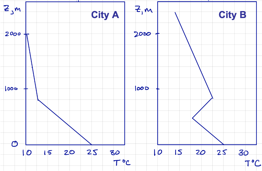
You are asked to assess the air quality in two cities A and B. The temperature profiles over each of the cities is shown below. Note that a parcel rising from the surface will start with the surface temperature 25 °C. Assume dry air.
- What is the mixing height (H) over each city?
- Based on the observed temperature profiles, estimate the stability class (A-F) for each city.
- Determine the vertically averaged velocity between z=0 and z=H. You are told that the wind speed 10 𝑚 above the surface is 𝑢=5 𝑚/𝑠. Note: the velocity profile follows the power law and the vertical average is given by:
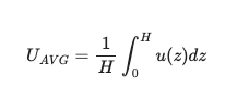
- What is the Dilution Rate (or ventilation coefficient) for each city?
- Which city is likely to have better air quality on this day?
- If both cities are 25 𝑘𝑚 across, what is the residence time over each?
Problem 3
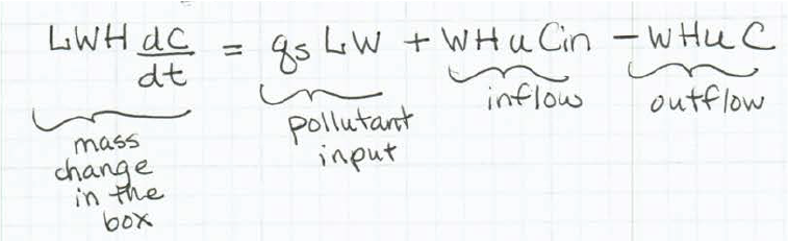
Consider an area-source box model for air pollution above a peninsula of land (see figure below). The length of the box is 30 km, its width is 100 km, and a radiation inversion restricts mixing to 100 m. Wind is blowing clean air into the long dimension of the box at 0.7 m/s. Between 4 and 6 pm there are 300,000 vehicles on the road, each being driven 25 km, and each emitting 5 g/km of CO.
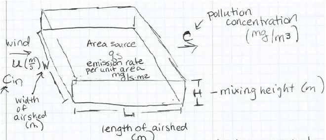
W = 100 km, L = 30 km, H=100 m, u = 0.7 m/s
- Find the average rate of CO emissions during this two-hour period (g CO/s per m^2 of land).
- Estimate the concentration of CO at 6 pm if there was no CO in the air at 4 pm. Assume that CO is conservative (does not decay or change) and that there is instantaneous and complete mixing in the box.
- Assume the windspeed is 0, and use the basic equation (below) to derive a relationship between CO and time and use it to find the CO over the peninsula at 6 pm.