5) Hydrology, Flooding and Statistics

You may be interested in the history of the Cedar River Watershed:

• History from Seattle Public Utilities
• History Link Article about Managing the Watershed

Homework 5

Problem 1: Average precipitation across a watershed (4 pts)

Choose one of the following methods for precipitation distribution.

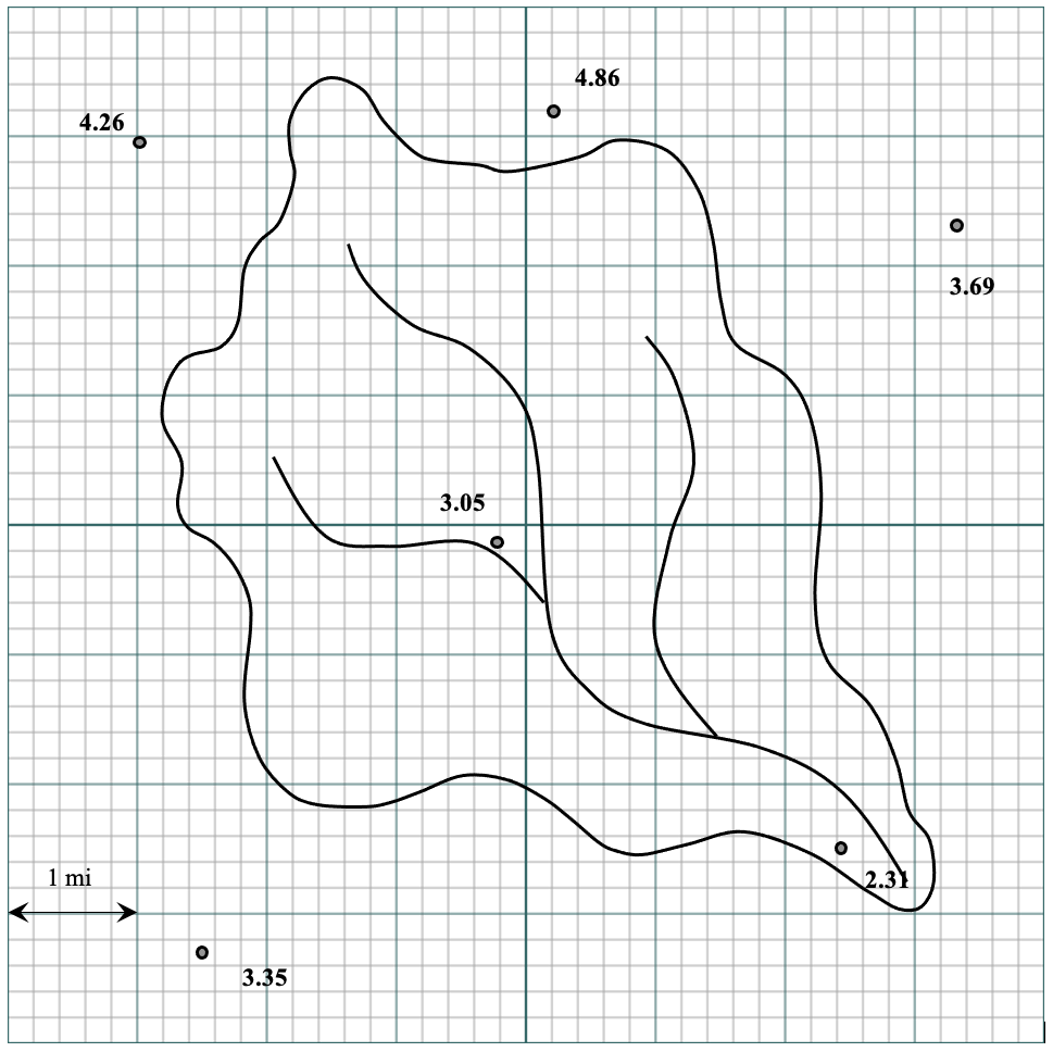
OPTION 1: In the map below and linked here, the recorded rainfall in inches is provided at six gauges in and around a watershed. Compute the mean areal rainfall over the watershed using the Theissen method (print this page, use a ruler, approximate using the squares, and scan to turn in with your homework). You will need to approximate on the number of squares in cases with fractions of squares, and any reasonable approximation is fine (just show your work).

OPTION 2: Follow Lab-3, but instead of the Olympics, extract a line of elevation along the center of the Cedar River Watershed. Note, you may use this elevation profile instead of extracting your own. Presuming precipitation follows the linear orographic precipitation model, determine the condensation rate (and presumed instantaneous rain rate) as a funtion of elevation. Note, it will be easiest if you smooth the slopes to assign between 3 and 4 rain rates over a range of elevations with similar general slope. Then, use the area at each elevation (easiest if you determine elevation bands) to determine the area-average rainfall (in mm) across the watershed. This excel sheet has information on elevation vs. area for the Cedar River. You may choose to import the area vs elevation from the excel sheet, or you can define elevation bands and sum the area within them in excel and then type/paste those area weights into your python notebook. Please show your work. Please extract your python notebook to PDF, or take screen shots and put it into a word document, before you turn it in.

Problem 2: Peak Flows and Flood Risk in the Cedar River Watershed (4 pts)

Use the annual peak flow values (in cubic feet per second, cfs) for the inflows to the Cedar River above the Chester Morse Reservoir available here. The original USGS data can be found here. You will see one value for each water year. Because a water year starts on October 1st of the prior year, you will sometimes seem two values that fall on the same calendar year. Some years do not have a peak flow listed due to gauging issues. These have been removed from the list. Rank the data from high to low. Use Weibull's plotting position Pr (X>=x): Pr = m/(n+1), where m in the rank of the discharge (with 1 indicating high flow) and n is your total number of observations. This gives you the exceedance probability. Use this to calculate the return period.

Following the example in lab 5-2, plot the data in log-probability space and estimate a best-fit-straight line through the data (you may do this by eye) to estimate what the 100-year flood is likely to be. Alternatively, you may iterate with the Weibull plotting to estimate. Compare with the Log-Pearson III formulas. Make sure to upload both your notebeook (.ipynb) and a .pdf version to canvas when you submit your homework.

Problem 3: Planning for final project video (2 pts)

Write 1-2 paragraphs of what you plan to do for your final project video. What will you cover? How many minutes will each sub-topic take? How will you present things visually? Feel free to include any sketches and diagrams and any questions you have at this point. Note that lecture notes for future class topics are now available in Canvas – also feel free to reach out to the professor or TA. This write-up will be peer reviewed as part of the next homework. Make sure that you have an electronic copy of your write-up that you will be able to post in a discussion forum on either Canvas or Slack for your classmates to access.