Lab 5-1: Turbulent fluxes and measures of stability#
Written by Eli Schwat - January 2024.
import xarray as xr
import numpy as np
import os
import urllib
import pandas as pd
import datetime as dt
import matplotlib.pyplot as plt
import altair as alt
SOS Data#
sos_file = "../data/sos_full_dataset_30min.nc"
sos_dataset = xr.open_dataset(sos_file)
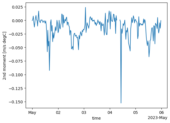
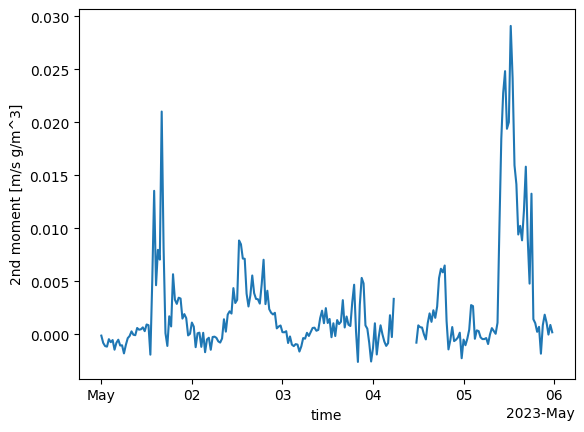
Check out the flux measurements in their native units#
sos_dataset['w_tc__3m_c'].sel(time=slice('20230501', '20230505')).plot()
[<matplotlib.lines.Line2D at 0x7ff06cfd7f50>]
sos_dataset['w_h2o__3m_c'].sel(time=slice('20230501', '20230505')).plot()
[<matplotlib.lines.Line2D at 0x7ff06df06690>]
Convert turbulent fluxes to energy units#
Converting turbulent latent heat flux measurements into energy flux units (\(W/m^2\))#
To convert w_h2o__3m_c (latent heat flux in \(g/m^2/s\)) to \(W/m^2\), we will use the latent heat of sublimation (the sum of the latent heats of fusion and vaporization, \(L_{sub} = 2590 J/g\)).
\(H_l = \) w_h2o__3m_c \( * L_{sub}\)
and the units work out like this : \(\frac{g}{m^2 s} * \frac{J}{g} = \frac{J}{m^2 s} = \frac{W}{m^2}\) (b/c 1 Watt = 1 Joule per second).
Converting turbulent sensible heat flux measurements into energy flux units (\(W/m^2\))#
To convert w_tc__3m_c (sensible heat flux in units \(K m/s\)) to \(W/m^2\), we will use the specific heat capacity of air (\(c_{p}^{air} = 1.005\) \(J/K/g\)) and the density of air (\(\rho_{air} = 1000 g / m^3\)). Note that we use the physical constants for air since it is air that is transporting heat away from the snowpack.
\(H_s = \) w_tc__3m_c \( * c_{p}^{air} * \rho_{air}\)
and the units work out like this: \(\frac{K m}{s} * \frac{J}{K g} * \frac{g}{m^3} = = \frac{W}{m^2}\)
latent_heat_sublimation = 2590 #J/g
latent_heat_flux = sos_dataset['w_h2o__3m_c'] * latent_heat_sublimation

specific_heat_capacity_air = 1.005 # J/K/g
air_density = 1000 # g/m^3
sensible_heat_flux = sos_dataset['w_tc__3m_c'] * specific_heat_capacity_air * air_density

# negating the measurements
sensible_heat_flux = sensible_heat_flux
sensible_heat_flux.sel(time=slice('20230501', '20230505')).plot(label='sensible')
latent_heat_flux.sel(time=slice('20230501', '20230505')).plot(label='latent')
plt.ylabel('Heat fluxes (W/m^2)')
plt.legend()
<matplotlib.legend.Legend at 0x7ff06c636110>
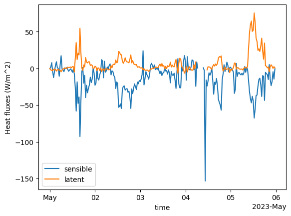
Why do we think sensible heat and latent heat have an inverse relationship?
Calculate Static Stability#
Stability is characterized with many different methods. One of the simpler methods is to characterize the “static stability” - the stabiliy of the atmopshere due to stratification alone. This is done by using the gradient in potential temperature,
Let’s calculate the static stability of the atmosphere throughout the entire season. We will use a finite difference approximation to the derivative above using measurements at the snow surface and at 3 meters. We will also ignore the fact that the snow depth is fluctuating.
T_vars = [
    'Tsurfpot_c', 'Tpot_3m_c',
]
stability_df = sos_dataset[
    T_vars

].to_dataframe()
stability_df.head()

stability_df['static_stability'] = (stability_df['Tpot_3m_c'] - stability_df['Tsurfpot_c'])/3
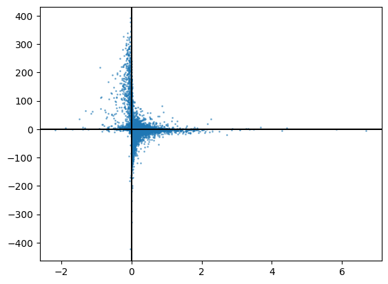
Compare static stability with sensible heat fluxes#
sensible_heat_flux = sensible_heat_flux.to_dataframe().join(stability_df[['static_stability']])
plt.scatter(
    sensible_heat_flux['static_stability'], sensible_heat_flux['w_tc__3m_c'],
    s=1, alpha=0.5
)
plt.axhline(0, color='black')
plt.axvline(0, color='black')
<matplotlib.lines.Line2D at 0x7ff06c523d10>
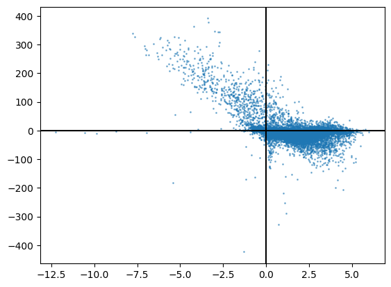
What pattern do we see? Why?
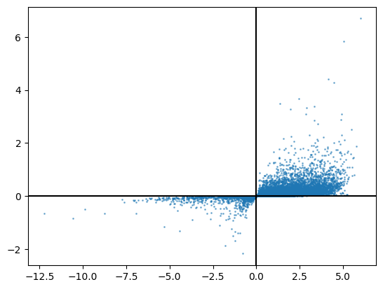
Calculate Dynamic Stability#
h = 3
g = 9.81
k = 0.4
theta_h = sos_dataset['Tpot_3m_c'] + 273.15
theta_s = sos_dataset['Tsurfpot_c'] + 273.15
u_h = sos_dataset['spd_3m_c']
Ri_bulk = g*h*(theta_h - theta_s)/(u_h**2 * 0.5*(theta_h + theta_s))
Ri_bulk.name = 'Ri_bulk'
sensible_heat_flux = sensible_heat_flux.join(Ri_bulk.to_dataframe())
sensible_heat_flux.head()
| w_tc__3m_c | static_stability | Ri_bulk | |
|---|---|---|---|
| time | |||
| 2022-11-01 00:00:00 | -1.798522 | 1.977773 | 0.833876 |
| 2022-11-01 00:30:00 | -8.952477 | 1.909485 | 0.103544 |
| 2022-11-01 01:00:00 | -0.394793 | 1.734680 | 0.209729 |
| 2022-11-01 01:30:00 | -7.073821 | 1.545715 | 0.094483 |
| 2022-11-01 02:00:00 | 8.566571 | 1.438609 | 0.067049 |
plt.scatter(
    sensible_heat_flux['Ri_bulk'], sensible_heat_flux['w_tc__3m_c'],
    s=1, alpha=0.5
)
plt.axhline(0, color='black')
plt.axvline(0, color='black')
<matplotlib.lines.Line2D at 0x7ff06c76bc90>
How does the relationship between w’T’ and dynamic stability (Ri) differ from the relationship between w’T’ and static stability (\(d \theta /dz\))
plt.scatter(
    sensible_heat_flux['static_stability'], sensible_heat_flux['Ri_bulk'],
    s=1, alpha=0.5
)
plt.axhline(0, color='black')
plt.axvline(0, color='black')
<matplotlib.lines.Line2D at 0x7ff06c5dbc50>
What pattern do we see? Why?