3) Mixing and dispersion in the atmosphere#
Lab 3: Gaussian Mixing and Smokestack plumes#
Download the lab and data files to your computer. Then, upload them to your JupyterHub following the instructions here.
Lab 3-5: BONUS, extra credit: Guassian Smokestack with an Inversion
Data: Sounding Data Jan 10
Data: Sounding Data Dec 26
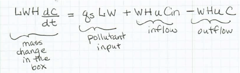
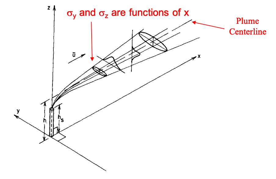
Graphic: Smokestack_gaussian_plume.png
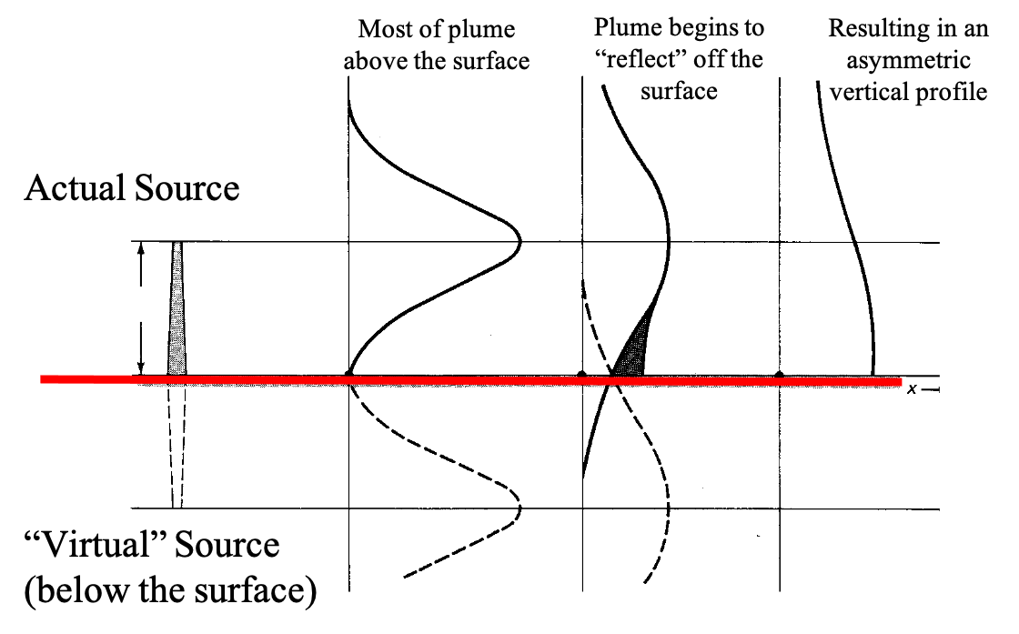
Graphic: Plume_reflection.png
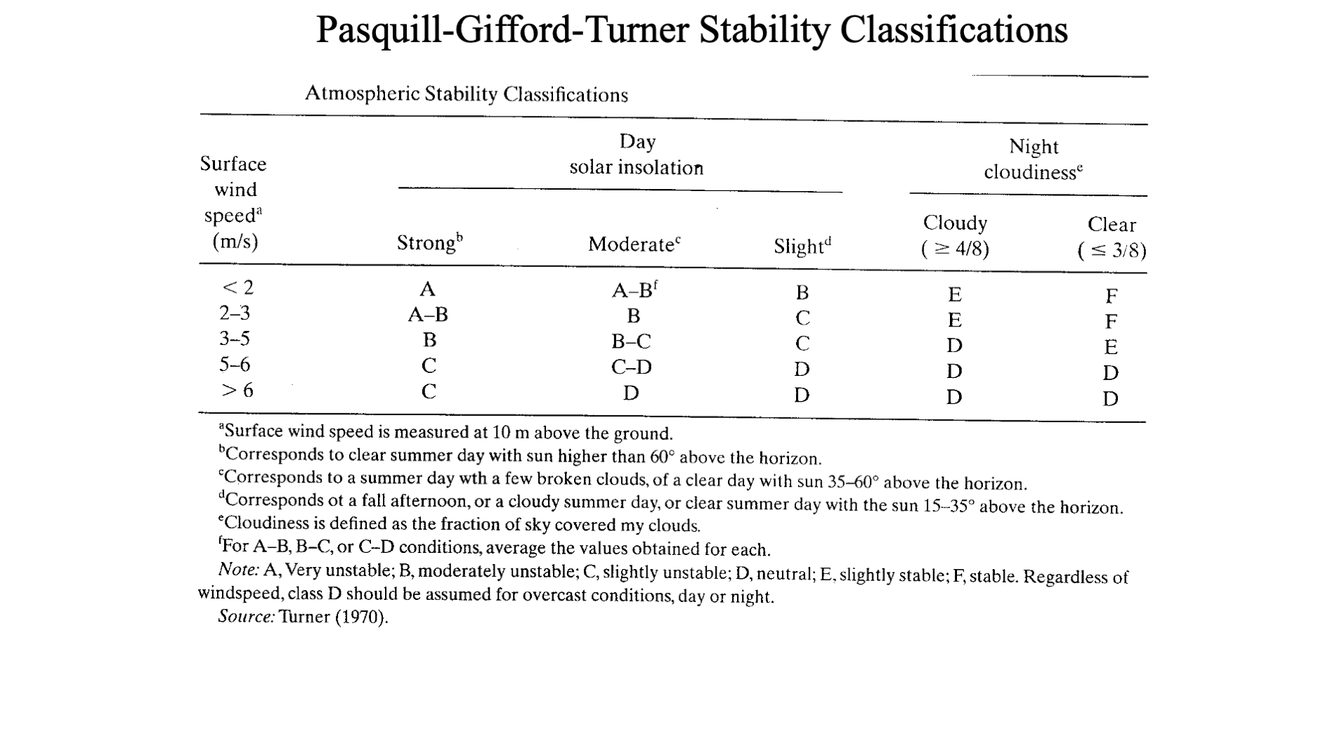
Graphic: Stability_classes.png
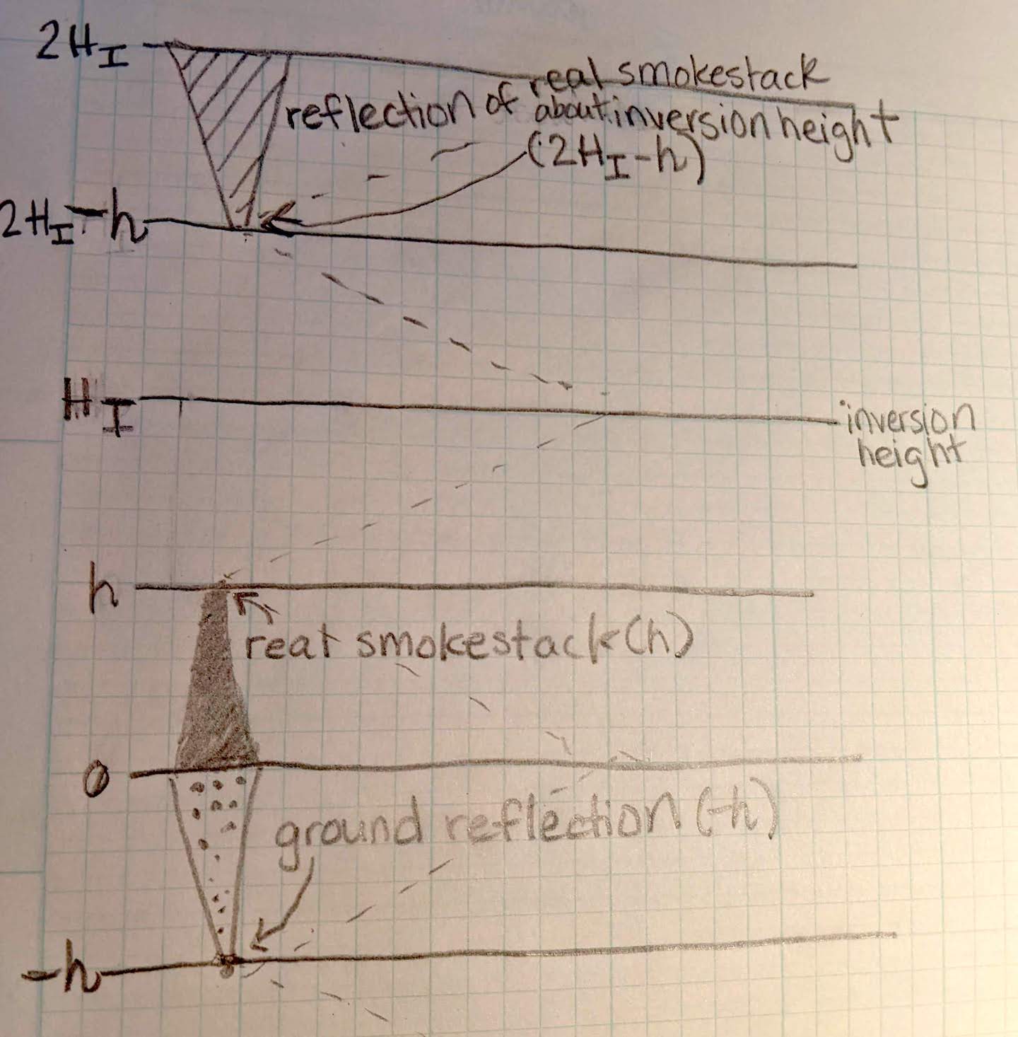
BONUS Graphic: Smokestack_oneReflection.jpg
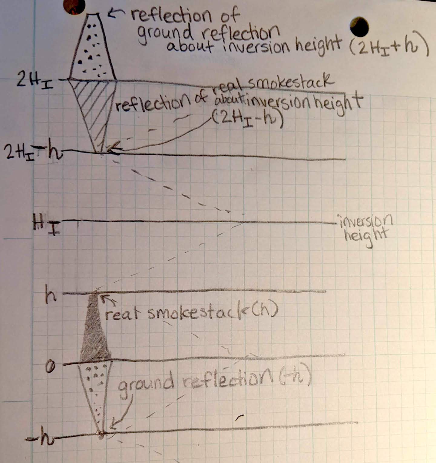
BONUS Graphic: Smokestack_2reflections.jpg
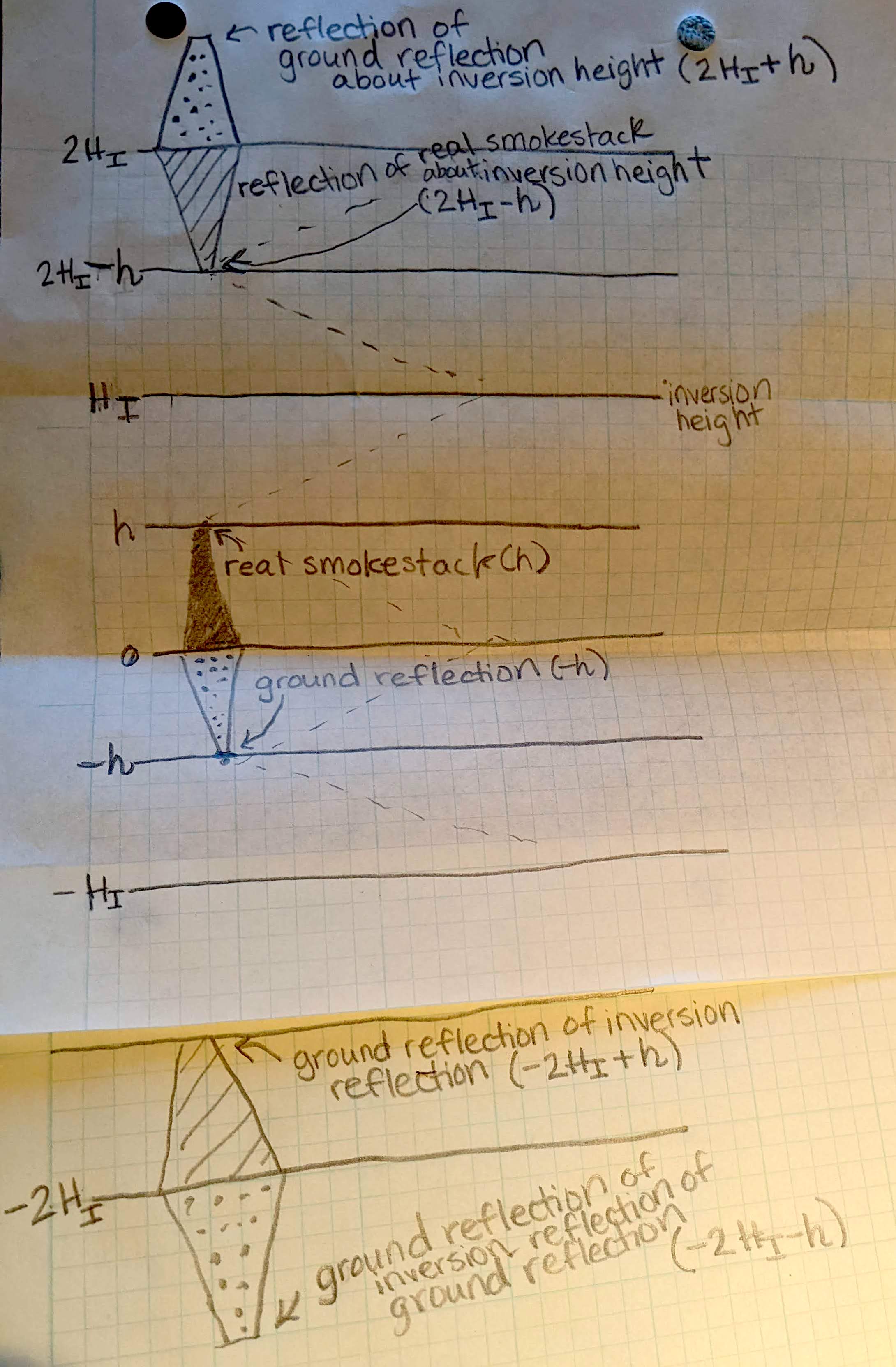
BONUS Graphic: Smokestacks_doublereflections.jpg
Homework 3:#
Problem 1#
On an overcast day with class C stability, the wind velocity at 10 m is 5 m/s. The emission rate of an atmospheric pollutant is 70 g/s from a stack having an effective height of 100 m. Assume rural conditions. (You will want to use the lab python notebooks to solve this problem.)
Estimate the center-line, ground-level concentration 25 km downwind from the stack, in micrograms per cubic meter.
Estimate the ground-level concentration 25 km downwind and 600 m from the stack center line, in micrograms per cubic meter.
Calculate and plot the centerline ground level concentration versus distance from the stack (C(x)).
From the plot, estimate the magnitude and location of the peak ground concentration.
How would the location and magnitude of the peak ground concentration change if the stack height was 125 𝑚? (Plot on the same axes)
Problem 2#
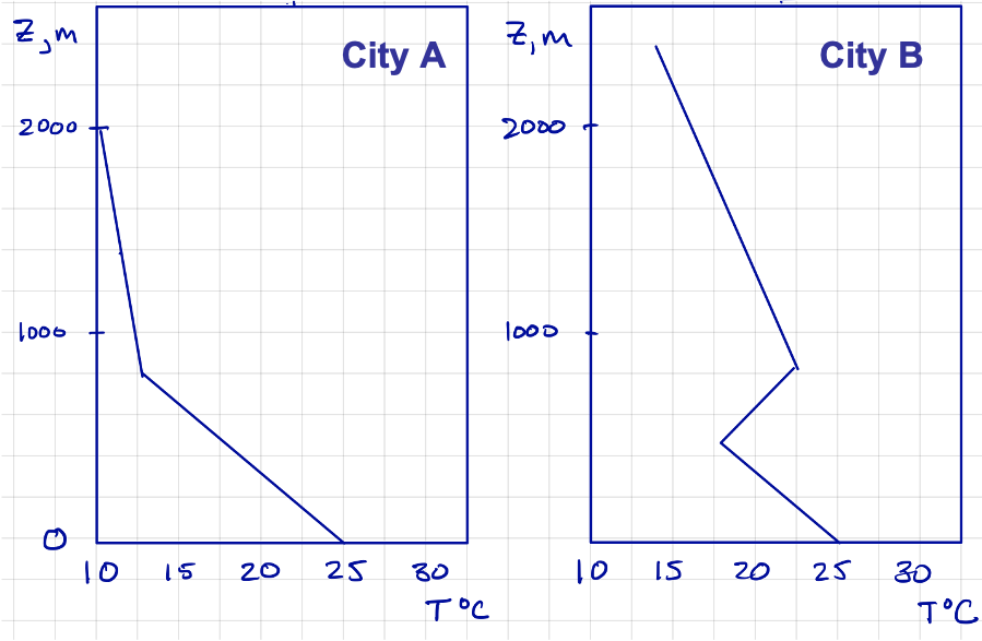
You are asked to assess the air quality in two cities A and B. The temperature profiles over each of the cities is shown below. Note that a parcel rising from the surface will start with the surface temperature 25 °C. Assume dry air.
What is the mixing height (H) over each city?
Based on the observed temperature profiles, estimate the stability class (A-F) for each city.
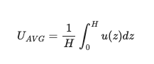
Determine the vertically averaged velocity between z=0 and z=H. You are told that the wind speed 10 𝑚 above the surface is 𝑢=6 𝑚/𝑠. Note: the velocity profile follows the power law and the vertical average is given by:
What is the Dilution Rate (or ventilation coefficient) for each city?
Which city is likely to have better air quality on this day?
If both cities are 30 𝑘𝑚 across, what is the residence time over each?
Problem 3#
Consider an area-source box model for air pollution above a peninsula of land (see figure below). The length of the box is 25 km, its width is 100 km, and a radiation inversion restricts mixing to 100 m. Wind is blowing clean air into the long dimension of the box at 1 m/s. Between 4 and 6 pm there are 400,000 vehicles on the road, each being driven 20 km, and each emitting 5 g/km of CO.
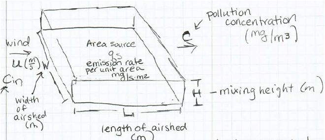
W = 100 km, L = 25 km, H=100 m, u = 1 m/s
Find the average rate of CO emissions during this two-hour period (g CO/s per m^2 of land).
Estimate the concentration of CO at 6 pm if there was no CO in the air at 4 pm. Assume that CO is conservative (does not decay or change) and that there is instantaneous and complete mixing in the box.
Assume the windspeed is 0, and use the basic equation (below) to derive a relationship between CO and time and use it to find the CO over the peninsula at 6 pm.